| [ < ] | [ > ] | [ << ] | [ Up ] | [ >> ] | [Top] | [Contents] | [Index] | [ ? ] |
3. Tutorial
An excellent user-written Asymptote tutorial is also available
from
http://www.artofproblemsolving.com/Wiki/index.php/Asymptote:_Basics
To draw a line from coordinate (0,0) to coordinate (100,100) using
Asymptote's interactive mode, type at the command prompt:
asy
draw((0,0)--(100,100));
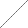
The units here are PostScript "big points"
(1 bp = 1/72 inch); -- means join with a linear segment.
In Asymptote coordinates like (0,0) and
(1000,100) are called pairs.
At this point you can type in further draw commands, which will be added
to the displayed figure, or type quit to exit interactive mode.
You can use the arrow keys in interactive mode to edit previous lines
(assuming that you have support for the GNU readline library
enabled). The tab key will automatically complete unambiguous words;
otherwise, hitting tab again will show the possible choices. Further
commands specific to interactive mode are described in Interactive mode.
In batch mode, Asymptote reads commands directly from a
file. To try this out, type
draw((0,0)--(100,100));
into a file, say test.asy. Then execute this file with the
MSDOS or UNIX command
asy -V test
MSDOS users can drag and drop the file onto the
Desktop asy icon or make Asymptote the
default application for files with the extension asy.
The -V option opens up a PostScript
viewer window so you can immediately view the encapsulated
PostScript output. By default the output will be written to the
file test.eps; the prefix of the output file may be changed with
the -o command-line option.
One can draw a line with more than two points and create a cyclic path like this square:
draw((0,0)--(100,0)--(100,100)--(0,100)--cycle);

It is often inconvenient to work directly with PostScript coordinates.
The next example draws a unit square scaled to width 101 bp and height
101 bp. The output is identical to that of the previous example.
size(101,101);
draw((0,0)--(1,0)--(1,1)--(0,1)--cycle);
For convenience, the path (0,0)--(1,0)--(1,1)--(0,1)--cycle
may be replaced with the predefined variable
unitsquare, or equivalently, box((0,0),(1,1)).
One can also specify the size in pt (1 pt = 1/72.27 inch),
cm, mm, or inches.
If 0 is given as a size argument, no restriction is made in that direction;
the overall scaling will be determined by the other direction
(see size):
size(0,3cm);
draw(unitsquare);

To make the user coordinates represent multiples of exactly 1cm:
unitsize(1cm);
draw(unitsquare);
One can also specify different x and y unit sizes:
unitsize(1cm,2cm);
draw(unitsquare);
Adding labels is easy in Asymptote; one specifies the
label as a double-quoted LaTeX string, a
coordinate, and an optional alignment direction:
size(0,3cm);
draw(unitsquare);
label("$A$",(0,0),SW);
label("$B$",(1,0),SE);
label("$C$",(1,1),NE);
label("$D$",(0,1),NW);

Asymptote uses the standard compass directions E=(1,0),
N=(0,1), NE=unit(N+E), and ENE=unit(E+NE), etc.,
which along with the directions up, down, right,
and left are defined as pairs in the Asymptote base
module plain. A user who has a local variable named E
may access the compass direction E by prefixing it with the name
of the module where it is defined: plain.E.
This example draws a path that approximates a quarter circle:
size(100,0);
draw((1,0){up}..{left}(0,1));
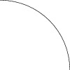
In general, a path is specified as a list of pairs (or other paths)
interconnected with
--, which denotes a straight line segment, or .., which
denotes a cubic spline.
Specifying a final node cycle creates a cyclic path that
connects smoothly back to the initial node, as in this approximation
(accurate to within 0.06%) of a unit circle:
path unitcircle=E..N..W..S..cycle;
Each interior node of a cubic spline may be given a
direction prefix or suffix {dir}: the direction of the pair
dir specifies the direction of the incoming or outgoing tangent,
respectively, to the curve at that node. Exterior nodes may be
given direction specifiers only on their interior side.
A cubic spline between the node z_0, with postcontrol point
c_0, and the node z_1, with precontrol point c_1,
is computed as the Bezier curve

As illustrated in the diagram below, the third-order midpoint (m_5)
constructed from two endpoints z_0 and z_1 and two control points
c_0 and c_1, is the point corresponding to t=1/2 on
the Bezier curve formed by the quadruple (z_0, c_0,
c_1, z_1). This allows one to recursively construct the
desired curve, by using the newly extracted third-order midpoint as an
endpoint and the respective second- and first-order midpoints as control
points:
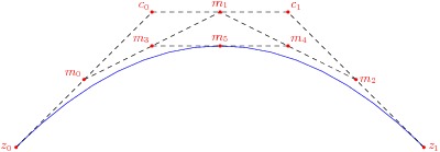
Here m_0, m_1 and m_2 are the first-order midpoints, m_3 and m_4 are the second-order midpoints, and m_5 is the third-order midpoint. The curve is then constructed by recursively applying the algorithm to (z_0, m_0, m_3, m_5) and (m_5, m_4, m_2, z_1).
In fact, an analogous property holds for points located at any fraction t in [0,1] of each segment, not just for midpoints (t=1/2).
The Bezier curve constructed in this manner has the following properties:
- It is entirely contained in the convex hull of the given four points.
- It starts heading from the first endpoint to the first control point and finishes heading from the second control point to the second endpoint.
The user can specify explicit control points between two nodes like this:
draw((0,0)..controls (0,100) and (100,100)..(100,0));
However, it is usually more convenient to just use the
.. operator, which tells Asymptote to choose its own
control points using the algorithms described in Donald Knuth's
monograph, The MetaFontbook, Chapter 14.
The user can still customize the guide (or path) by specifying
direction, tension, and curl values.
The higher the tension, the straighter the curve is, and the more it approximates a straight line. One can change the spline tension from its default value of 1 to any real value greater than or equal to 0.75 (cf. John D. Hobby, Discrete and Computational Geometry 1, 1986):
draw((100,0)..tension 2 ..(100,100)..(0,100));
draw((100,0)..tension 2 and 1 ..(100,100)..(0,100));
draw((100,0)..tension atleast 1 ..(100,100)..(0,100));
The curl parameter specifies the curvature at the endpoints of a path (0 means straight; the default value of 1 means approximately circular):
draw((100,0){curl 0}..(100,100)..{curl 0}(0,100));
The MetaPost ... path connector, which requests, when possible, an
inflection-free curve confined to a triangle defined by the
endpoints and directions, is implemented in Asymptote as the
convenient abbreviation :: for ..tension atleast 1 ..
(the ellipsis ... is used in Asymptote to indicate a
variable number of arguments; see section Rest arguments). For example,
compare
draw((0,0){up}..(100,25){right}..(200,0){down});

with
draw((0,0){up}::(100,25){right}::(200,0){down});

The --- connector is an abbreviation for ..tension atleast
infinity.. and the & connector concatenates two paths, after
first stripping off the last node of the first path (which normally
should coincide with the first node of the second path).
An Asymptote path, being connected, is equivalent to a
Postscript subpath. The ^^ binary operator, which
requests that the pen be moved (without drawing or affecting
endpoint curvatures) from the final point of the left-hand path to the
initial point of the right-hand path, may be used to group several
Asymptote paths into a path[] array (equivalent to a
PostScript path):
size(0,100);
path unitcircle=E..N..W..S..cycle;
path g=scale(2)*unitcircle;
filldraw(unitcircle^^g,evenodd+yellow,black);
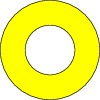
The PostScript even-odd fill rule here specifies that only the
region bounded between the two unit circles is filled (see fillrule).
In this example, the same effect can be achieved by using the default
zero winding number fill rule, if one is careful to alternate the
orientation of the paths:
filldraw(unitcircle^^reverse(g),yellow,black);
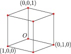
The ^^ operator is used by the box3d function in
three.asy to construct a two-dimensional projection of the edges of a 3D
cube, without retracing steps:
import three;

currentprojection=orthographic(5,4,2);

size(5cm);
size3(3cm,5cm,8cm);

draw(unitbox);

dot(unitbox,red);

label("$O$",(0,0,0),NW);
label("(1,0,0)",(1,0,0),S);
label("(0,1,0)",(0,1,0),E);
label("(0,0,1)",(0,0,1),Z);
See section graph (or the online Asymptote gallery and
external links posted at http://asymptote.sourceforge.net) for
further examples, including two and three-dimensional scientific
graphs. Additional examples have been posted by Philippe Ivaldi at
http://piprim.tuxfamily.org/asymptote/.
| [ < ] | [ > ] | [ << ] | [ Up ] | [ >> ] | [Top] | [Contents] | [Index] | [ ? ] |
