28.1 One-dimensional Interpolation

Octave supports several methods for one-dimensional interpolation, most of which are described in this section. Polynomial Interpolation and Interpolation on Scattered Data describe further methods.

Function File: yi = interp1 (x, y, xi)

Function File: yi = interp1 (…, method)

Function File: yi = interp1 (…, extrap)

Function File: pp = interp1 (…, 'pp')

One-dimensional interpolation. Interpolate y, defined at the points x, at the points xi. The sample points x must be strictly monotonic. If y is an array, treat the columns of y separately.

Method is one of:

'nearest'

Return the nearest neighbor.

'linear'

Linear interpolation from nearest neighbors

'pchip'

Piece-wise cubic hermite interpolating polynomial

'cubic'

Cubic interpolation from four nearest neighbors

'spline'

Cubic spline interpolation–smooth first and second derivatives throughout the curve

Appending '*' to the start of the above method forces interp1 to assume that x is uniformly spaced, and only x (1) and x (2) are referenced. This is usually faster, and is never slower. The default method is 'linear'.

If extrap is the string 'extrap', then extrapolate values beyond the endpoints. If extrap is a number, replace values beyond the endpoints with that number. If extrap is missing, assume NA.

If the string argument 'pp' is specified, then xi should not be supplied and interp1 returns the piece-wise polynomial that can later be used with ppval to evaluate the interpolation. There is an equivalence, such that ppval (interp1 (x, y, method, 'pp'), xi) == interp1 (x, y, xi, method, 'extrap').

An example of the use of interp1 is

xf = [0:0.05:10]; yf = sin (2*pi*xf/5); xp = [0:10]; yp = sin (2*pi*xp/5); lin = interp1 (xp, yp, xf); spl = interp1 (xp, yp, xf, "spline"); cub = interp1 (xp, yp, xf, "cubic"); near = interp1 (xp, yp, xf, "nearest"); plot (xf, yf, "r", xf, lin, "g", xf, spl, "b", xf, cub, "c", xf, near, "m", xp, yp, "r*"); legend ("original", "linear", "spline", "cubic", "nearest")

See also: interpft.

There are some important differences between the various interpolation methods. The 'spline' method enforces that both the first and second derivatives of the interpolated values have a continuous derivative, whereas the other methods do not. This means that the results of the 'spline' method are generally smoother. If the function to be interpolated is in fact smooth, then 'spline' will give excellent results. However, if the function to be evaluated is in some manner discontinuous, then 'pchip' interpolation might give better results.

This can be demonstrated by the code

t = -2:2;
dt = 1;
ti =-2:0.025:2;
dti = 0.025;
y = sign(t);
ys = interp1(t,y,ti,'spline');
yp = interp1(t,y,ti,'pchip');
ddys = diff(diff(ys)./dti)./dti;
ddyp = diff(diff(yp)./dti)./dti;
figure(1);
plot (ti, ys,'r-', ti, yp,'g-');
legend('spline','pchip',4);
figure(2);
plot (ti, ddys,'r+', ti, ddyp,'g*');
legend('spline','pchip');

The result of which can be seen in fig:interpderiv1 and fig:interpderiv2.

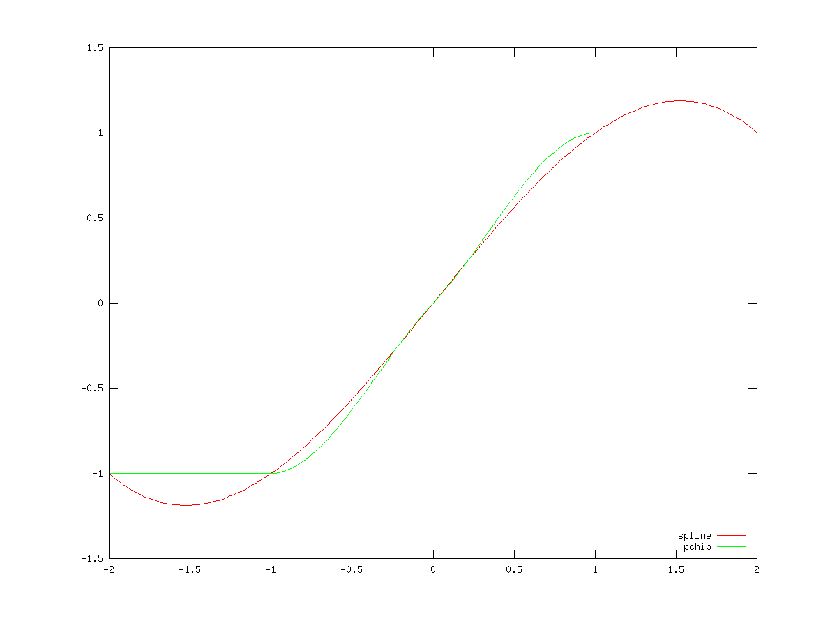
Figure 28.1: Comparison of 'pchip' and 'spline' interpolation methods for a step function

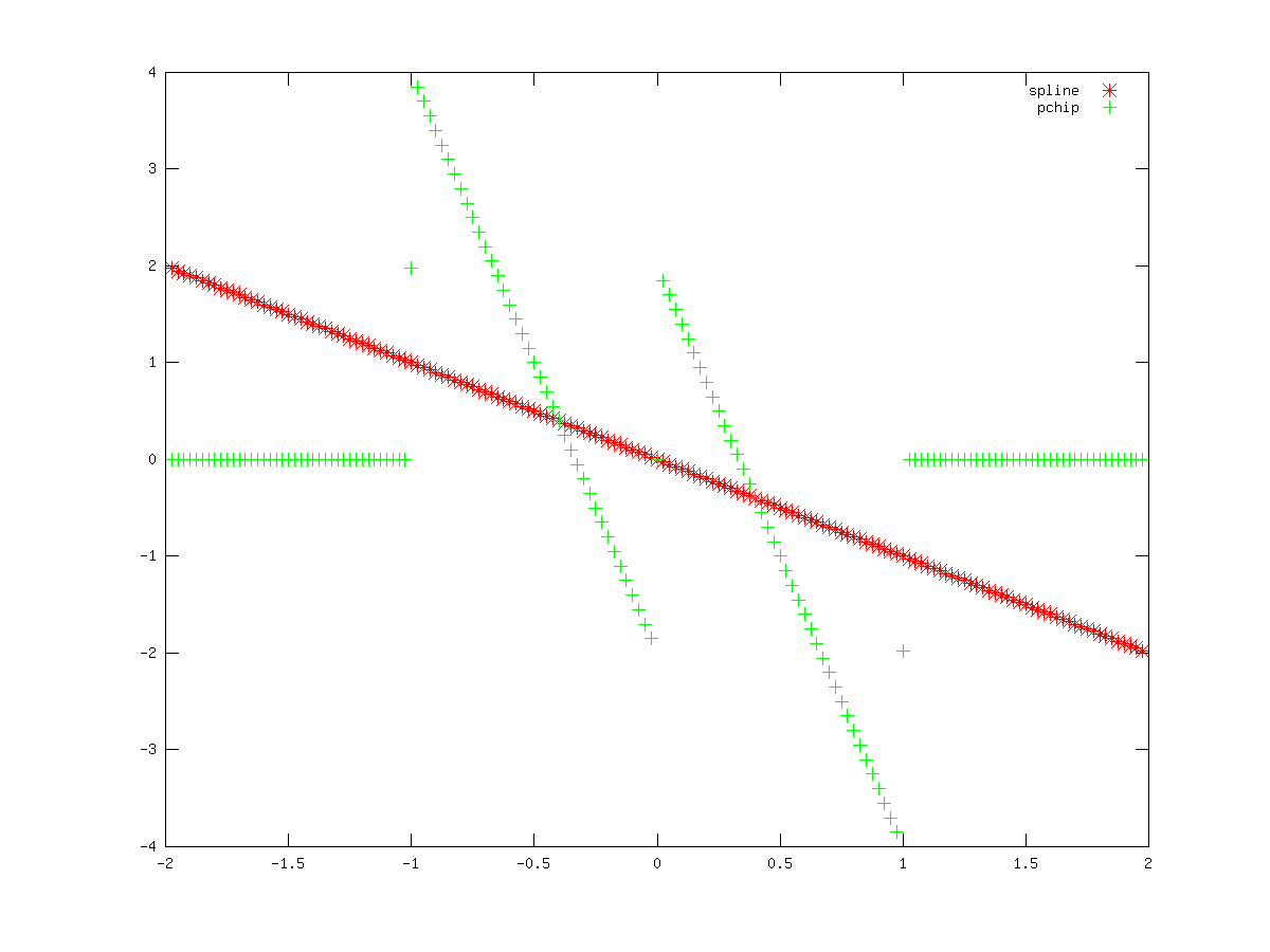
Figure 28.2: Comparison of the second derivative of the 'pchip' and 'spline' interpolation methods for a step function

A simplified version of interp1 that performs only linear interpolation is available in interp1q. This argument is slightly faster than interp1 as to performs little error checking.

Function File: yi = interp1q (x, y, xi)

One-dimensional linear interpolation without error checking. Interpolates y, defined at the points x, at the points xi. The sample points x must be a strictly monotonically increasing column vector. If y is an array, treat the columns of y separately. If y is a vector, it must be a column vector of the same length as x.

Values of xi beyond the endpoints of the interpolation result in NA being returned.

Note that the error checking is only a significant portion of the execution time of this interp1 if the size of the input arguments is relatively small. Therefore, the benefit of using interp1q is relatively small.

See also: interp1.

Fourier interpolation, is a resampling technique where a signal is converted to the frequency domain, padded with zeros and then reconverted to the time domain.

Function File: interpft (x, n)

Function File: interpft (x, n, dim)

Fourier interpolation. If x is a vector, then x is resampled with n points. The data in x is assumed to be equispaced. If x is an array, then operate along each column of the array separately. If dim is specified, then interpolate along the dimension dim.

interpft assumes that the interpolated function is periodic, and so assumptions are made about the end points of the interpolation.

See also: interp1.

There are two significant limitations on Fourier interpolation. Firstly, the function signal is assumed to be periodic, and so non-periodic signals will be poorly represented at the edges. Secondly, both the signal and its interpolation are required to be sampled at equispaced points. An example of the use of interpft is

t = 0 : 0.3 : pi; dt = t(2)-t(1);
n = length (t); k = 100;
ti = t(1) + [0 : k-1]*dt*n/k;
y = sin (4*t + 0.3) .* cos (3*t - 0.1);
yp = sin (4*ti + 0.3) .* cos (3*ti - 0.1);
plot (ti, yp, 'g', ti, interp1(t, y, ti, 'spline'), 'b', ...
      ti, interpft (y, k), 'c', t, y, 'r+');
legend ('sin(4t+0.3)cos(3t-0.1','spline','interpft','data');

which demonstrates the poor behavior of Fourier interpolation for non-periodic functions, as can be seen in fig:interpft.

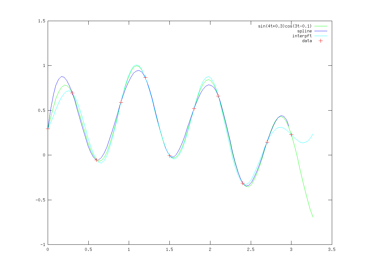
Figure 28.3: Comparison of interp1 and interpft for non-periodic data

In additional the support function spline and lookup that underlie the interp1 function can be called directly.

Function File: pp = spline (x, y)

Function File: yi = spline (x, y, xi)

Return the cubic spline interpolant of y at points x. If called with two arguments, spline returns the piece-wise polynomial pp that may later be used with ppval to evaluate the polynomial at specific points. If called with a third input argument, spline evaluates the spline at the points xi. There is an equivalence between ppval (spline (x, y), xi) and spline (x, y, xi).

The variable x must be a vector of length n, and y can be either a vector or array. In the case where y is a vector, it can have a length of either n or n + 2. If the length of y is n, then the 'not-a-knot' end condition is used. If the length of y is n + 2, then the first and last values of the vector y are the values of the first derivative of the cubic spline at the end-points.

If y is an array, then the size of y must have the form [s1, s2, …, sk, n] or [s1, s2, …, sk, n + 2]. The array is then reshaped internally to a matrix where the leading dimension is given by s1 * s2 * … * sk and each row of this matrix is then treated separately. Note that this is exactly the opposite treatment than interp1 and is done for compatibility.

See also: ppval, mkpp, unmkpp.

The lookup function is used by other interpolation functions to identify the points of the original data that are closest to the current point of interest.

Loadable Function: idx = lookup (table, y, opt)

Lookup values in a sorted table. Usually used as a prelude to interpolation.

If table is strictly increasing and idx = lookup (table, y), then table(idx(i)) <= y(i) < table(idx(i+1)) for all y(i) within the table. If y(i) < table (1) then idx(i) is 0. If y(i) >= table(end) then idx(i) is table(n).

If the table is strictly decreasing, then the tests are reversed. There are no guarantees for tables which are non-monotonic or are not strictly monotonic.

The algorithm used by lookup is standard binary search, with optimizations to speed up the case of partially ordered arrays (dense downsampling). In particular, looking up a single entry is of logarithmic complexity (unless a conversion occurs due to non-numeric or unequal types).

table and y can also be cell arrays of strings (or y can be a single string). In this case, string lookup is performed using lexicographical comparison.

If opts is specified, it shall be a string with letters indicating additional options. For numeric lookup, 'l' in opts indicates that the leftmost subinterval shall be extended to infinity (i.e., all indices at least 1), and 'r' indicates that the rightmost subinterval shall be extended to infinity (i.e., all indices at most n-1).

For string lookup, 'i' indicates case-insensitive comparison.