| [ < ] | [ > ] | [ << ] | [ Up ] | [ >> ] | [Top] | [Contents] | [Index] | [ ? ] |
7.31 graph3
This module implements three-dimensional versions of the
functions in graph.asy.
To draw an x axis in three dimensions, use the routine
void xaxis3(picture pic=currentpicture, Label L="", axis axis=YZZero,
            real xmin=-infinity, real xmax=infinity, pen p=currentpen,
            ticks3 ticks=NoTicks3, arrowbar3 arrow=None, bool above=false);
Analogous routines yaxis and zaxis can be used to draw
y and z axes in three dimensions.
There is also a routine for drawing all three axis:
void axes3(picture pic=currentpicture,
           Label xlabel="", Label ylabel="", Label zlabel="",
           triple min=(-infinity,-infinity,-infinity),
           triple max=(infinity,infinity,infinity),
           pen p=currentpen, arrowbar3 arrow=None);
The predefined three-dimensional axis types are
axis YZEquals(real y, real z, triple align=O, bool extend=false);
axis XZEquals(real x, real z, triple align=O, bool extend=false);
axis XYEquals(real x, real y, triple align=O, bool extend=false);
axis YZZero(triple align=O, bool extend=false);
axis XZZero(triple align=O, bool extend=false);
axis XYZero(triple align=O, bool extend=false);
axis Bounds(int type=Both, int type2=Both, triple align=O, bool extend=false);
The optional align parameter to these routines can be used to
specify the default axis and tick label alignments. The Bounds
axis accepts two type parameters, each of which must be one of
Min, Max, or Both. These parameters specify which
of the four possible three-dimensional bounding box edges should be drawn.
The three-dimensional tick options are NoTicks3, InTicks,
OutTicks, and InOutTicks. These specify the tick
directions for the Bounds axis type; other axis types inherit
the direction that would be used for the Bounds(Min,Min) axis.
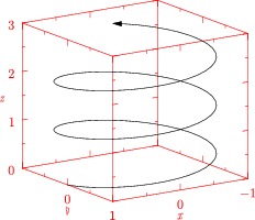
Here is an example of a helix and bounding box axes with ticks and axis labels, using orthographic projection:
import graph3;

size(0,200);
size3(200,IgnoreAspect);

currentprojection=orthographic(4,6,3);

real x(real t) {return cos(2pi*t);}
real y(real t) {return sin(2pi*t);}
real z(real t) {return t;}

path3 p=graph(x,y,z,0,2.7,operator ..);

draw(p,Arrow3);

scale(true);

xaxis3(XZ()*"$x$",Bounds(),red,InTicks(Label,2,2));
yaxis3(YZ()*"$y$",Bounds(),red,InTicks(beginlabel=false,Label,2,2));
zaxis3(XZ()*"$z$",Bounds(),red,InTicks);

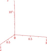
The next example illustrates three-dimensional x, y, and z axes, without autoscaling of the axis limits:
import graph3;

size(0,200);
size3(200,IgnoreAspect);

currentprojection=perspective(5,2,2);

scale(Linear,Linear,Log);

xaxis3("$x$",0,1,red,OutTicks(2,2));
yaxis3("$y$",0,1,red,OutTicks(2,2));
zaxis3("$z$",1,30,red,OutTicks(beginlabel=false));

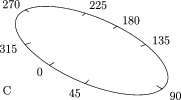
One can also place ticks along a general three-dimensional axis:
import graph3;

size(0,100);

path3 g=yscale3(2)*unitcircle3;
currentprojection=perspective(10,10,10);

axis(Label("C",position=0,align=15X),g,InTicks(endlabel=false,8,end=false),
     ticklocate(0,360,new real(real v) {
         path3 h=O--max(abs(max(g)),abs(min(g)))*dir(90,v);
         return intersect(g,h)[0];},
       new triple(real t) {return cross(dir(g,t),Z);}));

Surface plots of matrices and functions over the region
box(a,b) in the XY plane are also implemented:
surface surface(real[][] f, pair a, pair b, bool[][] cond={});
surface surface(real[][] f, pair a, pair b, splinetype splinetype,
                bool[][] cond={});
surface surface(real[][] f, real[] x, real[] y,
                splinetype splinetype=null, bool[][] cond={})
surface surface(triple[][] f, bool[][] cond={});
surface surface(real f(pair z), pair a, pair b, int nx=nmesh, int ny=nx,
                bool cond(pair z)=null);
surface surface(real f(pair z), pair a, pair b, int nx=nmesh, int ny=nx,
                splinetype splinetype, bool cond(pair z)=null);
surface surface(triple f(pair z), pair a, pair b, int nu=nmesh, int nv=nu,
                bool cond(pair z)=null);
The final version draws a parametric surface for a function
f(u,v) over the parameter space box(a,b),
as illustrated in the example parametricsurface.asy.
The boolean array or function cond can be used to control which
surface mesh cells are actually drawn (by default all mesh cells over
box(a,b) are drawn).
Surface lighting is illustrated in the example files
parametricsurface.asy and sinc.asy.
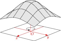
Lighting can be disabled by setting light=nolight, as in this example
of a Gaussian surface:
import graph3;

size(200,0);

currentprojection=perspective(10,8,4);

real f(pair z) {return 0.5+exp(-abs(z)^2);}

draw((-1,-1,0)--(1,-1,0)--(1,1,0)--(-1,1,0)--cycle);

draw(arc(0.12Z,0.2,90,60,90,25),ArcArrow3);

surface s=surface(f,(-1,-1),(1,1),nx=5,Spline);

xaxis3(Label("$x$"),red,Arrow3);
yaxis3(Label("$y$"),red,Arrow3);
zaxis3(XYZero(extend=true),red,Arrow3);

draw(s,lightgray,meshpen=black+thick(),nolight);

label("$O$",O,-Z+Y,red);

A mesh can be drawn without surface filling by specifying nullpen
for the surfacepen.
A vector field of nu\timesnv arrows on a
parametric surface f over box(a,b) can be drawn with the routine
picture vectorfield(path3 vector(pair v), triple f(pair z), pair a, pair b,
                    int nu=nmesh, int nv=nu, bool truesize=false,
                    real maxlength=truesize ? 0 : maxlength(f,a,b,nu,nv),
                    bool cond(pair z)=null, pen p=currentpen,
                    arrowbar3 arrow=Arrow3, margin3 margin=PenMargin3)
as illustrated in the examples vectorfield3.asy and
vectorfieldsphere.asy.
| [ < ] | [ > ] | [ << ] | [ Up ] | [ >> ] | [Top] | [Contents] | [Index] | [ ? ] |
